Understanding the Logistic Map and Fixed Points

Published on September 26, 2025 98 views

Have you ever wondered how complex behaviors in nature, like population growth, can emerge from surprisingly simple rules? Enter the Logistic Map, a mathematical model that’s a cornerstone in the study of chaos theory and complex systems.

It’s defined by the recursive equation:

$x_{t+1} = R \, (x_t - x_t^2)$

Here, $R$ is the growth rate, and $x_t$ represents the population (or system state) at a given time $t$ . The magic of this simple equation is how it can produce a stable, predictable outcome with one set of $R$ values, and complete chaos with others!

What is a Fixed Point?

In the context of the logistic map, a fixed point is a value that, once reached, remains constant in all subsequent iterations. It’s a point of stability where the system settles. Mathematically, a fixed point, $x^*$ , satisfies the condition:

$x^* = R (x^* - {x^*}^2)$

This means the value $x^*$ at time $t$ results in the exact same value at time $t+1$ .

Finding the Fixed Point: Step-by-Step

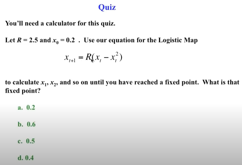
The quiz example provides a perfect scenario to demonstrate how a system finds its stability.

The Task:
We are given $R = 2.5$ and an initial value $x_0 = 0.2$ . We need to find the fixed point.

Method 1: Iterative Calculation (The Simulation Approach)

We’ll start with $x_0 = 0.2$ and calculate $x_1, x_2, x_3, \dots$ until the value stops changing significantly.

Iteration ( $t$ )	Calculation: $x_{t+1} = 2.5(x_t - x_t^2)$	Result ( $x_{t+1}$ )
t=0	$x_1 = 2.5 \times (0.2 - 0.2^2) = 2.5 \times (0.2 - 0.04)$	$x_1 = 0.4$
t=1	$x_2 = 2.5 \times (0.4 - 0.4^2) = 2.5 \times (0.4 - 0.16)$	$x_2 = 0.6$
t=2	$x_3 = 2.5 \times (0.6 - 0.6^2) = 2.5 \times (0.6 - 0.36)$	$x_3 = 0.6$

Since $x_2$ and $x_3$ are the same, the system has converged! The fixed point is 0.6.

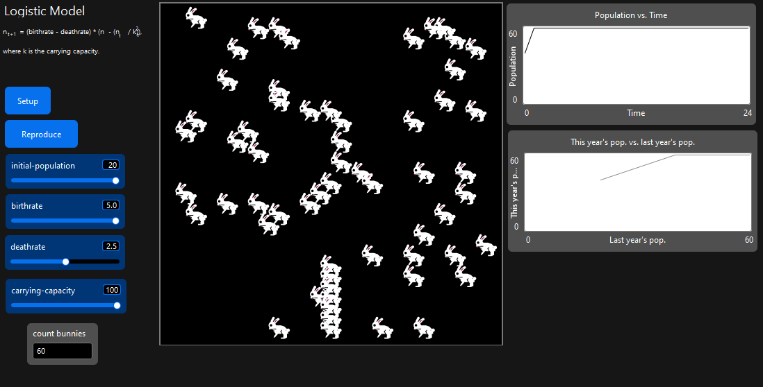
The visual from the NetLogo simulation (which models a similar logistic system) confirms this behavior: the population quickly rises from its initial state to a stable maximum.

Method 2: Analytical Calculation (The Fixed Point Formula)

To be absolutely sure, we can use the fixed point formula $x^* = R (x^* - {x^*}^2)$ and solve for $x^*$ using $R = 2.5$ .

Set the equation:

$x^* = 2.5 (x^* - {x^*}^2)$
Divide both sides by $x^*$ (assuming $x^* \ne 0$ ):

$1 = 2.5 (1 - x^*)$
Divide by $2.5$ (or multiply by $0.4$ ):

$\frac{1}{2.5} = 1 - x^*$

$0.4 = 1 - x^*$
Solve for $x^*$ (rearrange):

$x^* = 1 - 0.4$

$\mathbf{x^* = 0.6}$

Both methods confirm that the system stabilizes at 0.6.

Conclusion

This simple problem beautifully illustrates how a deterministic equation—the Logistic Map—can lead to a stable, predictable outcome, a fixed point. For $R=2.5$ and $x_0=0.2$ , the system quickly approaches and settles at 0.6 (Option b in the quiz).

The Logistic Map is a foundational tool in understanding how complex behaviors emerge from simple rules. If you increase the $R$ value, you start to see fascinating phenomena like period-doubling and eventually, chaos!