
The logistic map: a simple example
The logistic map is a tiny discrete formula that models population growth and is famous for showing how complex behavior can arise from simple rules. The map is:
![\[ x_{n+1} = r\, x_n (1 - x_n) \]](https://jeyhun.net/wp-content/ql-cache/quicklatex.com-63de843b72403ddc98647d332f070d6a_l3.png "Rendered by QuickLaTeX.com")
Here,  is the population fraction at step
  (values between 0 and 1), and
  is a growth parameter. Despite its simplicity, changing makes the map show rich behaviors.
Fixed points and stability
Fixed points (steady states) satisfy  . For the logistic map the fixed points solve:
![\[ x^* = r(x^* - {x^*}^2) \]](https://jeyhun.net/wp-content/ql-cache/quicklatex.com-bdf2f9cd054aaf834dc08fa6a11dfd86_l3.png "Rendered by QuickLaTeX.com")
Solving gives two basic fixed points:  and
and  (when
(when  ). Whether a fixed point is attracting or repelling depends on the slope of the map at that point.
Period doubling — the road to complexity
As you slowly increase the parameter , the system moves through stages:
- Stable fixed point: for small the population settles to a single value.
- Period-2: increase and the system alternates between two values (a cycle of length 2).
- Period-4, 8, 16, …: further increases cause the cycle period to double repeatedly.
- Chaos: after many doublings the behavior becomes aperiodic and highly sensitive — chaotic.
This sequence of doublings is called a period-doubling cascade, and it provides a universal route from order to chaos in many nonlinear systems.
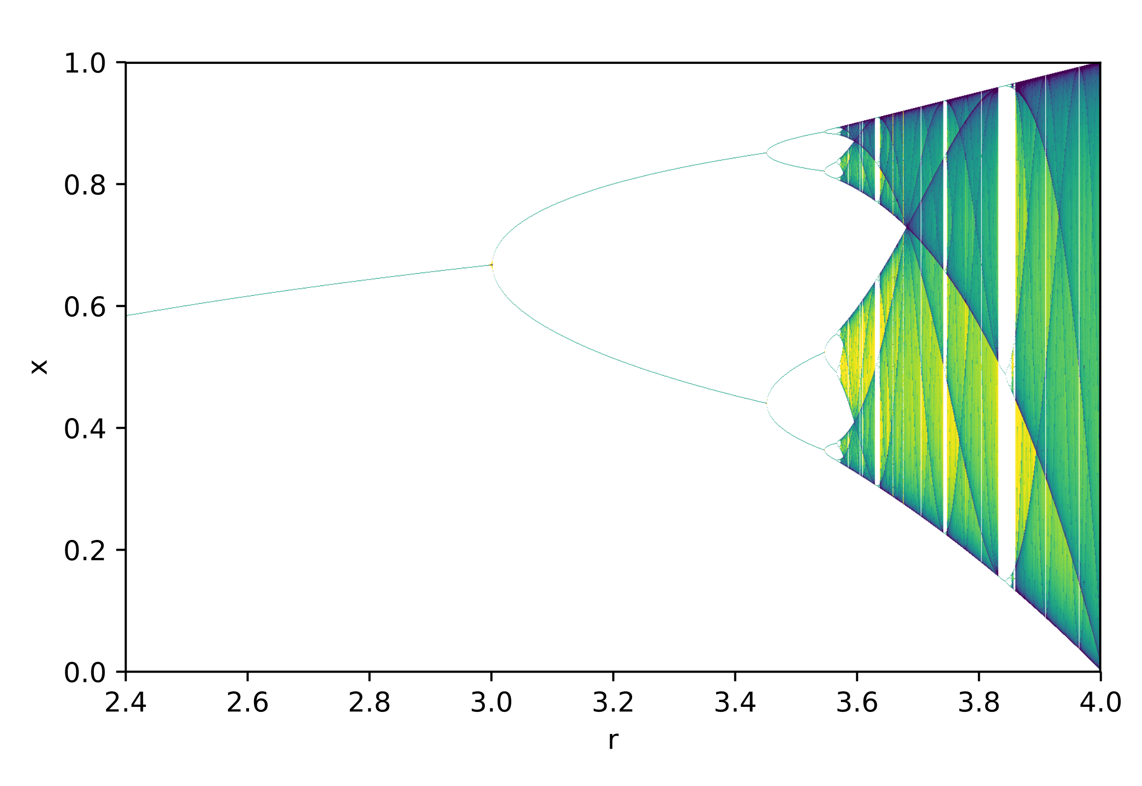
Bifurcation diagram — a picture of transitions
A bifurcation diagram is the usual visual tool to see the period-doubling route. It plots the parameter on the horizontal axis and the long-term values of  on the vertical axis. At low you see a single point (stable fixed point); then a fork (period-2), then more forks (period-4, etc.), and eventually a dense band indicating chaos. A bifurcation diagram neatly shows how small parameter changes reorganize the system’s long-term behavior.
Sensitivity to initial conditions
A hallmark of chaotic systems is sensitivity to initial conditions. Two trajectories that start almost identical—say  and
and  —remain close for a short time but eventually diverge exponentially fast in a chaotic regime. This makes long-term prediction effectively impossible even though the system is deterministic.
The period-doubling route to chaos appears in many areas:
- Biology — population dynamics and ecology
- Physics — fluid flows and lasers
- Electronics — nonlinear circuits
- Economics — cycles and irregular market behavior
Recognizing period doubling helps scientists understand how predictable systems can suddenly become unpredictable as some control parameter is changed.
Chaos is not randomness; it’s deterministic complexity. The period-doubling cascade and bifurcation diagrams give a clear, visual route from simple steady behavior to complex unpredictability, and sensitivity to initial conditions explains why prediction becomes hard. All of this arises from very simple mathematical rules—one of the most surprising and beautiful facts about nonlinear systems.
Real-World Bifurcations & Sudden Direction Changes
The period-doubling route and the “forking” of a single line in a bifurcation diagram are not mere mathematical curiosities — they appear in many natural, engineered, and social systems. Below is an explanation and concrete examples showing why the split can look abrupt and where you can find it in the real world.
Why the split appears sudden
A nonlinear system typically has one or more solutions for each parameter value. As a parameter changes, a solution can lose stability at a critical point: the solution itself still exists mathematically, but it no longer attracts trajectories. At the bifurcation point a new stable attractor (for example a 2-cycle) appears and immediately dominates observed behavior. To a viewer tracking only the stable attractor, this looks like a sudden jump — the old branch is still there but becomes repelling, so the system switches to a different regime.
If you zoom in on the branching region you usually find self-similar structure (fractals) and smaller nested bifurcations. The apparent abruptness is therefore a change in stability, not a discontinuity in the mathematical solutions.
Concrete examples
| Domain | System | Behavior (what bifurcates) | How the “split” looks in practice |
|---|---|---|---|
| Biology / Ecology | Population models (insects, microbes) | Stable population → periodic oscillations → chaos | A steady population begins regular boom-and-bust cycles (2, 4, 8, …) then irregular fluctuations |
| Physiology / Neuroscience | Heartbeat, neuronal firing | Regular rhythm → alternating patterns → irregular/chaotic firing | A consistent heartbeat can bifurcate into alternating strengths or arrhythmias |
| Fluid dynamics | Flow past obstacles, convection | Laminar → periodic vortex shedding → turbulence | Smooth flow develops repeating vortices, then chaotic eddies |
| Engineering / Electronics | Nonlinear circuits, oscillators | Stable output → periodic oscillations → chaotic oscillations | A constant voltage or simple sine output starts to oscillate more complexly |
| Economics / Social systems | Macro models, market feedback | Stable equilibrium → cycles (boom/bust) → irregular fluctuations | An economy may switch from steady growth to repeating cycles and then to erratic swings |
Historical example of a real-world bifurcation
One striking is the collapse of the Canadian cod fishery in 1992. For centuries, cod stocks off the coast of Newfoundland had been one of the richest fisheries in the world, supporting local communities and feeding international markets. Despite fluctuations, the population seemed stable and resilient.
In the mid-20th century, however, industrial fishing techniques such as factory trawlers and advanced sonar dramatically increased catch rates. Cod populations declined gradually at first, but managers assumed they would bounce back as they had in the past. What was not obvious is that the ecosystem was approaching a critical threshold — a bifurcation point.
Once that threshold was crossed in the late 1980s and early 1990s, the system’s stability vanished. Instead of recovering, cod stocks collapsed abruptly to a fraction of their historic levels. The Canadian government declared a moratorium on cod fishing in 1992, throwing more than 30,000 people out of work overnight in one of the largest sudden layoffs in modern history.
Even decades later, the cod population has not returned to its former equilibrium. The system shifted into a new regime where smaller fish and invertebrates dominate, preventing cod from regaining control of the ecosystem. This event illustrates how bifurcations in real life can look like sudden and irreversible “direction changes,” just as seen in mathematical bifurcation diagrams.
https://www.science.org/do/10.1126/science.abi8780/abs/Cod_fishing_1280x720.jpg

One-sentence takeaway
The dramatic split in a bifurcation diagram reflects a real change in stability: when a control parameter crosses a threshold, the system reorganizes into a new attractor — often abruptly — and this phenomenon is observed across biology, physics, engineering, and social sciences.
Downloads
NetLogo is a popular platform for agent-based modeling, designed so beginners can start easily while experts can tackle advanced research. It’s used in thousands of classrooms worldwide and featured in over 10,000 scientific publications.